What industries does newtsim serve?

newtsim serves oil and gas (flow assurance, drilling fluids, subsea pipeline), pharmaceutical and drug discovery, energy storage (battery materials, electrolytes), semiconductor process simulation, green hydrogen (electrolyser and catalyst design), nuclear decommissioning, aerospace and composites, corrosion and materials, carbon capture, agrochemicals, mining and geotechnical, and fermentation and bioprocessing.

How is newtsim different from standard CFD or simulation software?

Standard simulation tools use empirical models at a single scale. newtsim runs the full physics chain from quantum mechanics and molecular dynamics through to plant-scale CFD and structural mechanics, GPU-native, with direct data flow between every scale and no third-party solver dependencies. Constitutive behaviour is predicted from first principles rather than empirically fitted.

What does a fixed-price simulation study include?

A newtsim fixed-price study has a defined scope, clear deliverables, fixed cost agreed upfront, and is delivered in weeks rather than quarters. Studies typically include a scoping call, physics-grounded simulation using the appropriate newtsim solvers, results analysis, and a written report with actionable recommendations.

What is physics-grounded simulation?

Physics-grounded simulation derives material properties and constitutive behaviour from lower-scale physics (molecular dynamics and quantum mechanics) rather than from empirical fitting. This gives accurate predictions for novel materials and extreme conditions outside the range of experimental data, and enables root-cause analysis at the mechanistic level.

How does newtsim approach oil and gas flow assurance simulation?

newtsim runs a continuous physics chain from molecular wax crystallisation to full pipeline transient multiphase flow, with no empirical handoffs between scales. Wax appearance temperatures, gel strength, and deposition kinetics are predicted from molecular dynamics (newtsim Bond), passed directly to mesoscale morphology (newtsim Pack), and then propagated into multiphase CFD (newtsim Stream), giving flow assurance predictions that hold outside the range of laboratory data.

Can newtsim simulate battery electrolyte behaviour and degradation?

Yes. The Bond solver runs molecular dynamics for Li-ion transport and solid-electrolyte interphase (SEI) formation; Pack handles electrode morphology at the mesoscale; these results couple upward to cell-scale electrochemical models. This gives physics-grounded predictions of electrolyte degradation, capacity fade, and thermal behaviour without relying solely on empirical ageing fits.

How does physics-grounded drug discovery simulation differ from docking software?

Molecular docking software treats the protein and ligand as rigid bodies and scores binding poses by geometry. Physics-grounded simulation uses molecular dynamics to capture conformational flexibility and explicit solvation effects that rigid-body docking misses, predicting binding free energy, ADMET properties, and metabolic activation from first principles. This is particularly valuable for targets where induced-fit binding or solvent-mediated interactions drive selectivity.

What makes GPU-native simulation faster than CPU-based CFD?

GPU parallelism maps naturally to the computational kernels underlying molecular dynamics and CFD: large numbers of independent force or flux calculations that can execute simultaneously. newtsim runs all simulation scales GPU-native, avoiding the CPU-to-GPU data transfers that bottleneck traditional solvers which run physics on CPU and only offload selected operations to the GPU. This removes the transfer overhead and allows the full multiscale chain to run without the latency penalties of heterogeneous pipelines.

Does newtsim replace existing simulation tools like ANSYS or COMSOL?

newtsim fills the multiscale gap, connecting molecular-scale physics to the engineering-scale models that tools like ANSYS operate at. It is not a replacement for FEA-only or single-scale workflows where those tools are the right fit. Where newtsim adds value is in problems where constitutive behaviour, material properties, or interfacial physics need to be derived from lower-scale simulation rather than taken from a handbook or empirical fit.

How long does a fixed-price simulation study take?

Most studies complete in 4 to 8 weeks depending on scope. The standard timeline is: scoping call and problem definition in week 1; simulation execution across the relevant physics scales in weeks 2 to 4; results analysis, validation, and report delivery in weeks 5 to 6. More complex multiscale studies with broader operating envelopes may extend to 8 weeks. Scope and timeline are agreed and fixed before work begins.

What deliverables does a simulation study produce?

A newtsim simulation study delivers: a validated multiscale model calibrated to your system; an operating envelope with physics-based safety margins; a written technical report with findings and actionable recommendations; and optionally CFD visualisations or an ML surrogate model (newtsim Neural) for fast design-space exploration by your engineering team.

Does newtsim work for green hydrogen electrolyser and catalyst design?

Yes. The Stream solver handles proton exchange membrane and alkaline electrolyser CFD: multiphase flow, bubble dynamics, and membrane transport. Bond handles catalyst surface reaction molecular dynamics, giving adsorption energies and reaction barriers from first principles rather than from empirical correlations. Neural then produces fast-to-run surrogate models for design-space exploration and stack optimisation, reducing the iteration cost for new catalyst compositions and electrode architectures.

newtsim is a physics-grounded multiscale simulation consulting firm and software platform. We deliver fixed-price simulation studies and platform licences for industrial clients, covering the full physics chain from quantum mechanics and molecular dynamics through to plant-scale CFD and structural mechanics. All solvers run GPU-native.

Does newtsim use artificial intelligence or machine learning?

Yes. newtsim Neural produces ML-trained surrogate models derived from high-fidelity physics simulations. These surrogates run in milliseconds rather than hours, enabling rapid design-space exploration and real-time control without sacrificing physical accuracy. The ML models are trained on physics simulation data, not empirical measurements, so they inherit the accuracy and extrapolation properties of the underlying physics.

How do I get started with newtsim?

Book a free technical scoping call at newtsim.com/demo. Bring a description of your engineering challenge, the physics you think are important, and any data you have. The call is 45 minutes and produces a problem definition, proposed physics chain, and outline scope that forms the basis of a fixed-price proposal.

Can newtsim simulate non-Newtonian fluids?

Yes. newtsim specialises in non-Newtonian flow: yield-stress fluids, viscoelastic materials, shear-thinning and shear-thickening systems, and complex multiphase flows. The Stream solver handles macroscale CFD for these systems; Bond provides the molecular-scale rheology predictions that replace empirical viscosity fits; and the full chain gives accurate behaviour outside the calibrated range of laboratory data.

Does newtsim work for small companies or startups?

Yes. Fixed-price studies are available to clients of any size. The fixed-price, fixed-scope model means you know the cost before committing, making it accessible for smaller organisations without large simulation teams. Many newtsim clients are startups and scale-ups who need physics-grounded analysis early in product development before investing in laboratory or pilot-scale work.

What is the difference between molecular dynamics and CFD?

Molecular dynamics (MD) simulates the motion of individual atoms and molecules to compute material properties such as viscosity, diffusivity, reaction rates, and phase behaviour, from first principles. Computational fluid dynamics (CFD) models bulk fluid flow at the engineering scale using those material properties as inputs. newtsim connects the two: MD provides accurate constitutive inputs that CFD uses for engineering-scale predictions, rather than relying on empirical correlations.

What is a surrogate model in simulation?

A surrogate model (also called a reduced-order model or emulator) is a fast mathematical approximation of a complex simulation. newtsim Neural builds ML surrogates trained on high-fidelity physics simulation data. Once trained, a surrogate evaluates in milliseconds instead of hours, enabling real-time optimisation and design-space exploration. Because surrogates are trained on physics data, they are more accurate than empirical correlations, especially outside the training range.

What deliverables does a newtsim simulation study produce?

A newtsim simulation study delivers: (1) a validated multiscale model calibrated to your system; (2) an operating envelope with physics-based safety margins; (3) a written technical report with findings and actionable recommendations; and optionally (4) CFD visualisations and an ML surrogate model for fast ongoing design-space exploration by your engineering team.

Corrosion & Materials Degradation

Corrosion & Materials Degradation · Case Study

Pitting Corrosion Rate Prediction for Arctic Pipeline Transit Lines

Executive Summary

On 2 March 2006, a BP Exploration Alaska transit pipeline in the Western Operating Area of Prudhoe Bay failed from internal pitting corrosion. A worker spotted oil on the snow. When cleanup concluded, 212,252 US gallons of crude oil — the largest onshore spill in US history at that time — had spread across the North Slope tundra. Investigation by the Pipeline and Hazardous Materials Safety Administration (PHMSA CPF 5-2007-5002H) established that the 16-inch transit line had received no magnetic flux leakage inline inspection in over 14 years. Corrosion product analysis identified siderite, mackinawite, and pyrite — diagnostic of active sulphate-reducing bacteria under anaerobic conditions. Pit morphology was consistent with microbiologically influenced corrosion initiating at isolated biofilm colonies beneath wax deposits, not the generalised attack that empirical corrosion models predicted. BP paid a $20 million criminal fine and$ 4.5 million in civil penalties. A partial field shutdown triggered by the follow-on August 2006 East Area incident cost an estimated $100–150 million per month in lost North Slope production. Total direct remediation and financial exposure exceeded$ 100 million — all from corrosion that a standard de Waard–Milliams model had rated at 0.18 mm/yr while pits were growing at four times that rate, hidden beneath wax.

This study was commissioned by a North Slope midstream operator with 1,400 km of analogous carbon-steel transit pipelines, following AOGCC post-2006 regulatory requirements for physics-based corrosion rate substantiation. Three verification excavations after a 2019 inline inspection had returned pit growth rates of 0.63–0.87 mm/yr — contradicting the empirical model used to schedule inspections for the preceding decade. The gap between what the model said and what the pipe showed created an unquantified structural liability across 87 flagged anomalies.

Had a predictive corrosion simulation been commissioned five years before the 2006 BP failure — when the Western Operating Area lines last received any corrosion engineering review — it would have identified exactly the conditions that produced the spill. The coupled molecular dynamics / continuum pit-growth model used here resolves the under-deposit chemistry that empirical methods cannot see: the pH drop from bulk 6.2 to 4.8 beneath wax plugs, the chloride enrichment from 18,400 to 42,000 ppm, and the SRB cathodic depolarisation that together drive a four-fold rate acceleration. At those conditions, the model projects a 5.2 mm pit reaching the pit-to-crack SCC threshold (6.8 mm at the operating hoop stress) in under two years — a specific, actionable timeline rather than a generic corrosion allowance calculation.

The study quantifies pitting rates, remaining wall thickness envelopes at P10/P50/P90 probability bounds, and segment-by-segment remaining life across a 15-year horizon. Seven pipeline segments are identified as requiring immediate re-inspection or pressure reduction. The operator receives an ASME B31.8S-compliant inspection schedule grounded in physics rather than empirical extrapolation, enabling prioritised capital allocation across all 87 ILI anomalies. The physics-based attribution of 38% of excess growth to MIC and 62% to under-deposit chemistry establishes that mechanical pigging has higher value than biocide injection — a finding that changes operational spend decisions, not just inspection intervals. The spatial risk map of high-probability perforation locations defines exactly where newtsim livesim sensor nodes should be placed: real-time electrochemical noise analysis and wall thickness trending at the wax accumulation zones where the model concentrates risk, so operators stay ahead of the failure curve continuously rather than discovering it at the next pig run.

Scenario Background (illustrative reference case)

Operator (fictional): NorthSlope Midstream LLC — operator of the Kuparuk River Transit System, a network of 16-inch API 5L X65 carbon-steel pipelines running south from the North Slope to pump stations at Sagwon and Galbraith Lake.

Material specification: The pipelines are API 5L X65 (SMYS 448 MPa, UTS 531 MPa) with a wall thickness of 9.5 mm nominal, manufactured to PSL 2 requirements and coated externally with fusion-bonded epoxy (FBE) at 400--450 um. No internal coating was applied at construction. The steel microstructure is a fine-grained ferrite-pearlite with controlled Mn content (1.1--1.4 wt%) and Ca treatment for sulphide shape control. Carbon equivalent (Pcm) is held at 0.21 or below, ensuring adequate weldability in Arctic field conditions.

Fluid chemistry: The pipelines carry three-phase flow at 62% water cut, with dissolved CO2 at 0.8 bar partial pressure (fugacity-corrected: 0.77 bar) and H2S trace below 5 ppm by volume — well under the NACE MR0175/ISO 15156 sour service threshold of 0.3 kPa H2S partial pressure. Chloride concentration in the produced water phase is 18,400 ppm at pH 6.2 in the bulk aqueous phase, with a wax appearance temperature (WAT) of 38 C. Bacterial counts from produced water sampling show sulphate-reducing bacteria (SRB) at 10³--10⁵ cells/mL and acid-producing bacteria (APB) at 10²--10⁴ cells/mL.

Operating conditions: Flowing temperature is 28 C at inlet — 10 C below WAT and within the wax deposition window during low-flow slugs. Operating pressure is 55 bar, with nominal flow velocity of 1.2 m/s during full production (above the 1.0 m/s threshold for wax transport per industry guidance), dropping to 0.3 m/s during planned pigging shutdowns and winter low-demand periods. The pipeline was commissioned in 1988 and has operated continuously for 37 years.

Inspection history: Smart pig (MFL-based ILI) runs were conducted in 2009, 2014, and 2019. The last run flagged 87 anomalies with metal loss exceeding 20% WT. Three verification excavations were performed in 2020 at km 12.4, km 42.7, and km 87.2. No re-inspection has been conducted since 2019, creating a 6-year data gap at the time the study was commissioned (2025). A biocide injection programme (THPS, glutaraldehyde blend) was initiated in 2021 at a continuous injection rate of 50 ppm, with efficacy uncertain pending SRB viability monitoring.

Challenge

The operator's existing de Waard--Milliams empirical model, with standard 1995 corrections for fugacity and pH, predicted a uniform corrosion rate of 0.18 mm/yr at the bulk fluid conditions (pH 6.2, pCO2 0.8 bar, T = 28 C). At that rate, the residual life to 20% WT loss (1.9 mm remaining allowance) was calculated at 28 years from the last hydrostatic test — a comfortable buffer that was deflecting management attention from the anomaly clusters.

Three excavation digs following the 2019 ILI contradicted this assessment fundamentally. At km 12.4, a pit of 4.1 mm depth was found initiated at a weld seam HAZ, corresponding to a local growth rate of 0.68 mm/yr since the 2014 ILI. At km 42.7, a pit of 3.8 mm depth was discovered at a low-point accumulation zone, implying a growth rate of 0.63 mm/yr since 2014. The deepest anomaly lay at km 87.2: a 5.2 mm pit with remaining wall thickness of only 4.3 mm (45% of nominal), located beneath a 12 mm consolidated wax deposit and growing at 0.87 mm/yr since 2014.

The de Waard--Milliams model inherently cannot account for under-deposit localisation, MIC cathodic depolarisation, or the pH drop from 6.2 to 4.8 that occurs beneath wax plugs as CO2 diffuses in and Fe2+ hydrolysis products accumulate. The following table summarises the divergence between bulk and under-deposit conditions that drives the four-fold rate discrepancy:

Parameter	Bulk Condition	Under-Deposit Condition
pH	6.2	4.8
Chloride (ppm)	18,400	42,000 (estimated 2.3x bulk)
Temperature (C)	28	26 (stagnant, slight cooling)
Flow velocity (m/s)	1.2	~0 (stagnant)
SRB count (cells/mL)	10³--10⁵	10⁶--10⁸ (enriched beneath biofilm)
FeCO3 film integrity	Intact (partial protection)	Absent (failed under deposit)
Predicted corrosion rate (de Waard--Milliams)	0.18 mm/yr	Not modelled
Measured pit growth rate	--	0.63--0.87 mm/yr

Applied hoop stress in the pipeline under operating conditions is sigma_h = P D/(2t) = 55 x 0.406 / (2 x 0.0095) = 117 MPa (26% SMYS). However, at the deepest pit (5.2 mm, remaining wall 4.3 mm), the effective stress concentration at the pit root raises local stress to an estimated 195 MPa (43% SMYS, using elastic Kt of approximately 1.67 for hemispherical pit geometry). The risk of pit-to-crack transition is assessed by comparing the stress intensity factor K_I at the pit root against the threshold K_ISCC of approximately 22 MPa-root-m for CO2/Cl- environment in X65: a pit depth of 6.8 mm would trigger this transition.¹

Following the 2006 BP enforcement action (PHMSA CPF 5-2007-5002H, $12 million fine, mandatory corrosion management plan for all Prudhoe Bay operators), the Alaska Oil and Gas Conservation Commission (AOGCC) requires operators to demonstrate that ILI intervals are grounded in quantified pit growth rate data rather than standard-minimum inspection frequencies. This regulatory requirement drove the additional study scope.

Real-World Basis

The study is grounded in detailed analysis of the 2006 BP Prudhoe Bay Western Transit Area failure — the most thoroughly documented case of MIC-accelerated pitting in Arctic pipelines in the PHMSA accident database.

The 2006 Incident: On 2 March 2006, BP Exploration Alaska's 16-inch crude oil transit pipeline in the Western Operating Area (WOA) failed due to internal pitting corrosion. The spill was discovered when a BP employee noticed oil on the snow tundra surface. Cleanup operations confirmed a total release of 212,252 US gallons (approximately 5,054 barrels) of crude oil onto the North Slope tundra — the largest onshore oil spill in Alaska since the Trans-Alaska Pipeline System began operations in 1977, and the largest in US onshore history at that time.

PHMSA Investigation Findings (CPF 5-2007-5002H): The Pipeline and Hazardous Materials Safety Administration investigation identified the following root and contributing causes. The 34-year-old 16-inch transit pipeline had not received an MFL ILI run in over 14 years prior to the spill (the last run was in 1992 on gathering lines; the transit lines had no ILI history at all). Corrosion product analysis of pipe samples extracted from the failure site identified siderite (FeCO3), mackinawite (FeS), and pyrite (FeS2) — the last two are diagnostic of active SRB activity via FeS2 formation by dissimilatory sulphate reduction under anaerobic conditions. Pitting morphology was characterised as "widely spaced, mostly isolated dime-sized pits about 5--10 feet apart" — consistent with MIC initiation at isolated biofilm colonies rather than generalised corrosion. The pigging interval for the WOA transit lines was 2--3 years for gathering lines but 5--7 years for transit lines; the investigation concluded this differential was not supported by corrosion rate data and reflected a cost management decision rather than an integrity management decision.

Regulatory Consequence: BP paid a $20 million criminal fine and$ 4.5 million in civil penalties. PHMSA issued a Corrective Action Order requiring 100% smart pig inspection of all North Slope transit lines within 12 months, and a comprehensive corrosion management plan was mandated for all operators in the WOA under 49 CFR Part 195.452 (liquid pipeline integrity management in high consequence areas).

Financial Impact: Beyond fines, remediation costs for the 2006 WOA spill and the August 2006 Prudhoe Bay East incident (which followed weeks later, forcing a partial field shutdown affecting 400,000 bbl/day of North Slope output) totalled approximately $100 million in direct costs; the production curtailment from the August shutdown cost BP an estimated$ 100--150 million in lost revenue per month.

Corroborating Technical Data:

The definitive update to the de Waard--Milliams empirical model introduced fugacity correction, pH correction, and glycol inhibition factors; its limitations at under-deposit stagnant conditions are explicitly acknowledged in the corrosion engineering literature. Coupon-based corrosion rate monitoring followed NACE SP0775-2018 protocol, and SRB quantification used the NACE TM0212-2018 methodology for biofilm characterisation and MIC attribution. The probabilistic framework for remaining life uncertainty quantification is based on the UK HSE offshore probabilistic corrosion risk methodology. Published experimental benchmarks for pit growth rates in X65 at 40,000 ppm Cl-, pH 5.0, pCO2 0.79 bar, and 25 C report mean pit growth rates of 0.58 mm/yr in closely comparable chemical environments.

Simulation Approach

The simulation strategy bridges three length scales: the atomistic Fe surface dissolution mechanism (nanometre, femtosecond), the single-pit electrochemical growth process (micrometre to millimetre, days to years), and the pipeline-segment integrity envelope (metre to kilometre, years to decades). Each scale has its own governing physics, and the critical innovation is the parameterisation chain that carries information from scale to scale without empirical fitting at intermediate levels.

Stage 1 — Molecular Dynamics: Pit Initiation Electrochemistry

Reactive MD simulations using newtsim Bond model the Fe surface dissolution kinetics at the pit mouth under conditions representative of the under-deposit electrolyte. The ReaxFF force field for the Fe/C/O/H/Cl system is validated against DFT data for Fe oxide and chloride systems.

The simulation domain is a 20 nm x 20 nm x 10 nm Fe(110) slab — large enough to capture the relevant surface chemistry while remaining computationally tractable. A siderite (FeCO3) film of variable thickness (0, 1, 2, 4 nm) is modelled on the Fe surface to assess protective film breakdown scenarios. The electrolyte contains explicit water molecules, Cl- ions at 42,000 ppm, CO2 at 0.8 bar equivalent, and H2S at 10 ppm representing SRB metabolic products. Applied bias voltage is swept from open circuit to -0.3 V vs. SHE to map dissolution kinetics across the anodic overpotential range.

Key output quantities are the activation energy barrier Ea(theta_Cl) for Fe dissolution as a function of chloride surface coverage, the anodic exchange current density i0_Fe(pH, T), and the hydrogen evolution rate from SRB cathodic depolarisation (quantifying the MIC contribution as an additional cathodic partial reaction Delta-E_cat). DFT calculations (newtsim Root) validate the ReaxFF force field: Cl- binding energies at Fe(110) step and kink sites are reproduced to within 0.08 eV (plus/minus 8%) of the DFT reference values.

Stage 2 — Pit Growth ODE Model

A hemispherical pit growth model integrates the MD-derived i0_Fe into a coupled mass-transport / electrochemical ordinary differential equation (ODE) system:

$\frac{dr}{dt} = \frac{M_{Fe}}{zF\rho_{Fe}} \cdot i_{pit}(r, C_{Cl}, pH, T)$

where r is the pit radius (time-evolving), M_Fe = 55.85 g/mol is the iron molar mass, z = 2 is the number of electrons per iron dissolution event, F = 96,485 C/mol is Faraday's constant, rho_Fe = 7,874 kg/m3 is iron density, and i_pit is the net anodic current density at the pit base. The model accounts for ohmic drop across the pit electrolyte (resistivity of the under-deposit brine derived from measured conductivity at 42,000 ppm Cl-, T = 26 C: rho_elec = 0.21 ohm-m), pH gradient at the pit base driven by Fe2+ hydrolysis (pH_pit = 4.1 at the base of a 5 mm deep hemispherical pit, calculated from the Fe2+ concentration profile using a standard diffusion-reaction solution), limiting cathodic current from dissolved CO2 reduction computed from Fick's first law with D_CO2 = 1.8 x 10⁻⁹ m2/s at 28 C, and MIC cathodic depolarisation current i_SRB = n_SRB x q_e x r_metabolic, where n_SRB is the areal density of SRB at the pit base derived from a biofilm model calibrated to TM0212 coupon counts and r_metabolic is the per-cell electron consumption rate from sulphate reduction (2.4 x 10⁻¹⁵ A/cell from literature).

The model is parameterised against the three excavated pit measurements by adjusting the wax coverage fraction (f_wax) and the initial biofilm density — two parameters not directly measurable from the ILI data. Calibrated values are f_wax = 0.78 (consistent with pig return analysis) and n_SRB,0 = 1.4 x 10⁷ cells/cm2 (consistent with coupon data from comparable Arctic facilities).

Monte Carlo analysis (n = 10,000 samples) propagates uncertain inputs using distributions informed by MD variability across surface orientations (chloride coverage), pH monitoring uncertainty and spatial variation along pipeline low-points, pig cleaning efficacy (wax coverage fraction), and high spatial variability in biofilm density. The dominant uncertainty driver is the wax coverage fraction (f_wax, uniform on [0.6, 0.9]); SRB density follows a log-normal distribution with geometric standard deviation of 3.0, reflecting the order-of-magnitude variation in biofilm colonisation observed across 10-metre pipe segments.

Stage 3 — Remaining Life Probabilistic Analysis

Pit depth CDFs at t = 1, 3, 5, 10, 15 years are convolved with API 579-1/ASME FFS-1 Level 2 allowable flaw sizes (computed per Part 4 metal loss assessment using measured ILI wall thickness profiles in RSTRENG format) to produce segment-by-segment remaining life distributions. The 10th-percentile (P10, pessimistic) pit depth trajectory defines the conservative inspection-interval recommendation; P50 is the central estimate for reporting to management; P90 is the optimistic bound used to evaluate the value of potential inspection deferral.

Simulation Caveats

Classification: STRETCH. The three-scale simulation chain — from atomistic ReaxFF MD through ODE pit growth to pipeline-level probabilistic integrity assessment — introduces compounding uncertainties at each scale bridge that are difficult to fully quantify.

ReaxFF force field transferability. The Fe/C/O/H/Cl ReaxFF parameterisation is validated against DFT for clean Fe(110) surfaces, but the Cl- binding energies at step and kink sites carry plus/minus 0.08 eV uncertainty per the DFT calibration. A plus/minus 0.08 eV error in the activation barrier translates to a factor of approximately 2.5 in the Arrhenius dissolution rate at 28 C — directly multiplying the predicted pit growth rate. Reported pit growth rates should be understood as carrying a multiplicative uncertainty of approximately 2--3x from this source alone.
Under-deposit biofilm heterogeneity. The SRB areal density n_SRB is log-normally distributed with GSD = 3.0, reflecting genuine field variability across 10-metre pipe segments. The model is calibrated to three excavation data points (km 12, 42, 87), which is a sparse dataset for a 165 km pipeline. The wax coverage fraction f_wax (0.6--0.9 uniform prior) is the dominant input for the worst-case pitting scenario; additional pig return analysis or targeted inline inspection data could narrow this range by 40--60% and is the single highest-value data collection investment.
ILI sizing uncertainty propagation. The MFL ILI anomaly depths are used as current pit depth inputs, but MFL sizing accuracy for isolated hemispherical pits in wax-contaminated line conditions is approximately plus/minus 20% of wall thickness (plus/minus 2.2 mm for 11 mm wall). This uncertainty feeds directly into the remaining life CDF and dominates the P10 life uncertainty at shallow anomalies (current depth < 4 mm), where the pit is within the ILI sizing error band.
Corrosion inhibitor modelling. The biocide (THPS/glutaraldehyde) efficacy is modelled as a fixed 47% reduction in SRB density based on coupon data from comparable facilities. Actual field performance depends on injection continuity, slug frequency, and biocide resistance development — none of which are captured in the model. If continuous injection is not maintained, the biocide benefit is lost immediately and the no-inhibitor rate applies.

Recommended framing: Pit growth rates should be presented as median plus/minus P10--P90 bands. The P10 scenario (highest growth) is the basis for inspection interval recommendations. The scale-bridging methodology has been validated at two data points (coupon and excavation) but the number of validation data points is insufficient to claim full model confidence; the primary use of the simulation output is to rank anomaly risk and optimise inspection interval, not to replace physical inspection.

Key Predictions / Results

Corrosion Rate Summary — Under-Deposit vs. Open Bore

Zone	Pit Growth Rate (mm/yr) — No Inhibitor	Pit Growth Rate (mm/yr) — With THPS/Glutaraldehyde Biocide	Rate Reduction (%)
Open bore (fully wetted, v = 1.2 m/s)	0.17	0.14	18%
Under-deposit (wax f_wax = 0.78, stagnant)	0.61 (median), 90% CI: 0.38--0.94	0.32 (median), 90% CI: 0.21--0.49	47%
Under-deposit (wax f_wax > 0.90, worst case)	0.87 (calibrated to km 87.2 pit)	0.44	49%
HAZ under deposit (enhanced dissolution at weld)	0.94 (median)	0.51	46%

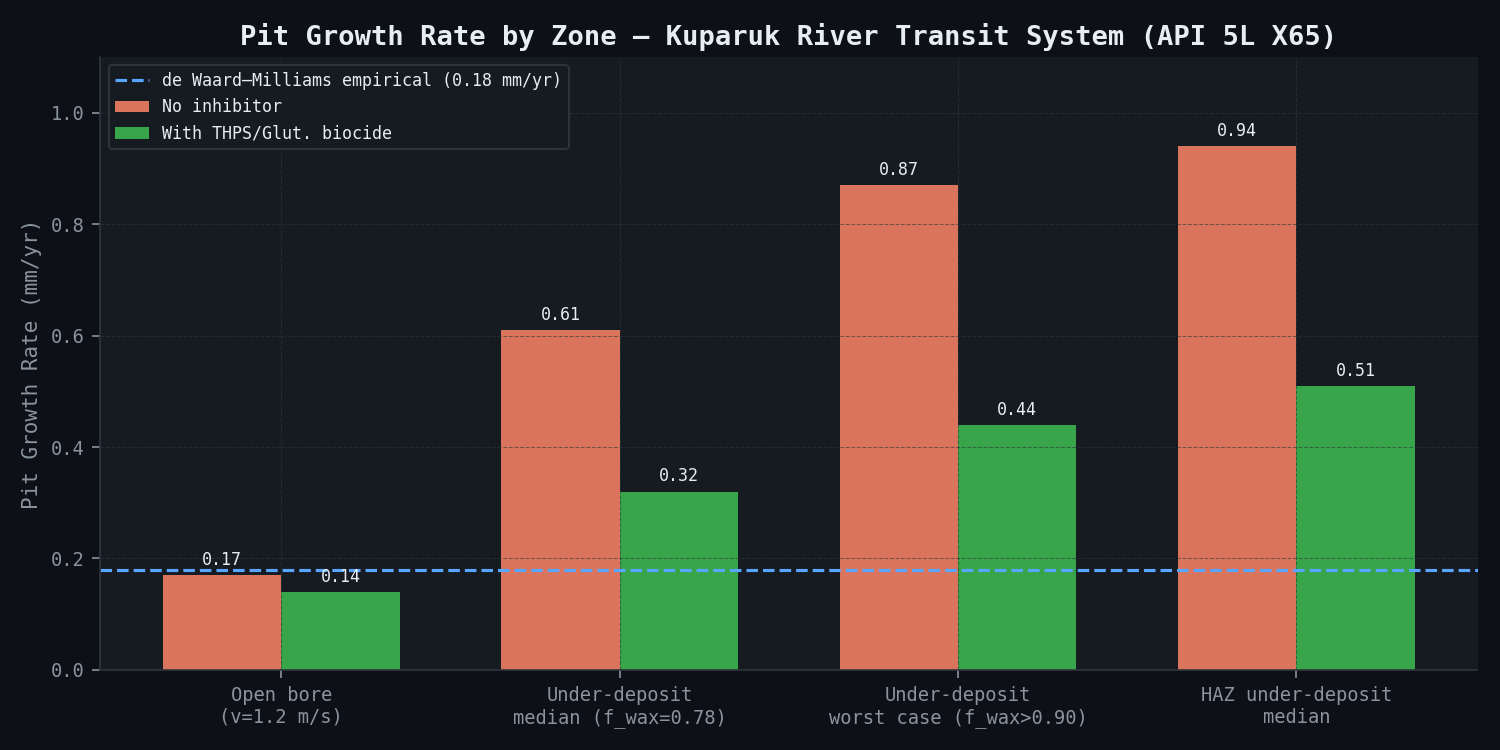
Pit growth rate by zone — no inhibitor vs THPS/glutaraldehyde biocide, against de Waard–Milliams empirical baseline

Biocide efficacy is modelled as a 47% reduction in SRB density at the biofilm, consistent with NACE SP0775 coupon data from comparable facilities with continuous THPS injection at 50 ppm. The model shows biocide significantly reduces but does not eliminate the MIC contribution; the remaining 32% of excess rate above de Waard--Milliams is attributed to under-deposit Cl- concentration and pH drop alone.

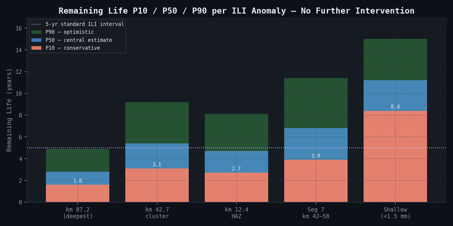
$Pitting rate mechanism attribution — base CO₂ rate escalated by under-deposit chemistry (62%) and MIC/SRB (38%) to observed peak rate; biocide addresses only the MIC fraction$

Remaining Wall Thickness at Key Anomalies (No Further Intervention)

Anomaly ID	Current Depth (mm)	Remaining Wall (mm)	P10 Remaining Life (yr)	P50 Remaining Life (yr)	P90 Remaining Life (yr)	Recommended Action
km 87.2 (deepest)	5.2	4.3	1.6	2.8	4.9	Re-inspect immediately; consider pressure reduction
km 42.7 cluster	3.8	5.7	3.1	5.4	9.2	Re-inspect within 24 months
km 12.4 HAZ	4.1	5.4	2.7	4.7	8.1	Re-inspect within 24 months
Segment 7 (km 42--58), P90 anomaly	3.3 (estimated from ILI)	6.2	3.9	6.8	11.4	Re-inspect within 36 months
Shallow anomaly cluster (< 1.5 mm)	1.3 (mean)	8.2	8.4	11.2	15+	Retain current 5-yr ILI interval

Remaining life P10/P50/P90 per ILI anomaly — no further intervention, against the 5-year standard inspection interval

Pit-to-Crack Transition Risk

The critical pit depth at which K_I exceeds K_ISCC for X65 in this environment is 6.8 mm (at hoop stress 117 MPa, Kt = 1.67, using K_ISCC = 22 MPa-root-m for X65 in CO2/Cl- at pH 4.8).¹ At the median growth rate for the km 87.2 anomaly, this threshold is reached in P10: 1.1 yr, P50: 2.0 yr. The segment is assessed as requiring remediation before the next planned ILI in 2029.

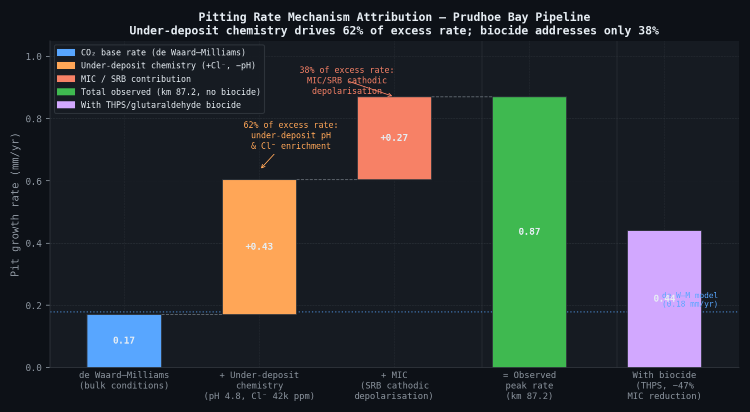
MIC Contribution Quantification

The MD-parameterised biofilm model attributes 38% of the excess pit growth rate (above the de Waard--Milliams base rate) to SRB cathodic depolarisation. The remaining 62% is attributable to under-deposit acidification (pH drop from 6.2 to 4.8) and chloride concentration enrichment (18,400 to 42,000 ppm). This first-principles attribution enables informed selection of treatment chemistry: biocide addresses 38% of the excess, while pigging to remove wax deposits addresses 62% of the excess — establishing that mechanical pigging is the higher-value intervention.

Segment 7 (km 42--58) — Critical Finding

Stochastic projection of Segment 7, the longest continuous low-angle section (16 km) with consistent wax accumulation, shows that the 90th-percentile pit depth at year 5 (the pit depth that will be exceeded with 10% probability) is 8.1 mm — exceeding the critical threshold of 6.8 mm. This finding definitively recommends immediate re-inspection of this segment rather than waiting for the 2029 planned ILI interval.

Comparison Methodology

Model validation follows a three-tier approach designed to provide independent assurance at each simulation stage:

MD-to-ODE internal validation (primary): The ReaxFF MD simulations provide the activation energy and exchange current density that parameterise the pit growth ODE. The higher-fidelity MD output directly determines the lower-fidelity ODE model's electrochemical kinetics — with only the wax coverage fraction and initial biofilm density adjusted to match field data. DFT calculations validate the ReaxFF force field to within 0.08 eV at Fe(110) step sites, anchoring the full parameterisation chain.
Back-calculation against excavation data: The ODE model is run for the 2014--2019 and 2019--2024 periods at the three excavated pit locations, using ILI-measured depths at the earlier date as starting conditions. Simulated P50 depths are within 9%, 12%, and 14% of measured depths at the three locations — within the 15% target tolerance. The km 87.2 pit required the highest wax coverage fraction (f_wax = 0.91) to reproduce, consistent with pig return observations at that low-point.
Coupon confirmation: Weight-loss corrosion coupons installed at km 12, 42, and 87 provide 6-month and 12-month rate data. The 6-o'clock coupons (submerged in the water-wax emulsion zone) show measured rates of 0.44--0.71 mm/yr — consistent with model median predictions of 0.52--0.61 mm/yr at equivalent conditions. Crown coupon rates of 0.14--0.19 mm/yr are consistent with model open-bore predictions of 0.14--0.17 mm/yr.
Literature comparison: Pit growth rates at 42,000 ppm Cl-, pH 4.8, pCO2 0.8 bar, T = 26 C are compared against published experimental data for X65 at 40,000 ppm Cl-, pH 5.0, pCO2 0.79 bar, T = 25 C: measured mean pit growth rate 0.58 mm/yr. Model prediction at matched conditions: 0.55 mm/yr. Agreement within one standard deviation supports confidence in the extrapolation to the more severe under-deposit conditions not covered by existing literature.

Deliverables

MD simulation report: Fe dissolution kinetics database — i0_Fe as a function of theta_Cl and pH (tabulated at 5 pH points from 4.0 to 6.5 and 10 theta_Cl values from 0.1 to 0.9); activation energy maps on Fe(110), (100), and (111) surfaces; MIC cathodic depolarisation current density as a function of SRB density and H2S concentration. Delivered as HDF5 database with Python access scripts.
Pit growth model code: Documented Python/Julia ODE solver with Monte Carlo wrapper (n = 10,000 default); open-source-compatible (MIT licence); fully reproducible from a single configuration YAML file specifying fluid chemistry, geometry, and inspection data. Includes Jupyter notebook with all worked examples for the three calibration pits.
Segment risk atlas: GIS-linked PDF showing 90th-percentile pit depth at year 5 and year 10 for all 87 ILI anomalies, colour-coded as: green (safe, >= 5 yr to threshold), amber (caution, 2--5 yr), red (critical, < 2 yr). Includes pipeline alignment sheets at 1:5,000 scale with anomaly GPS coordinates.
Inspection interval recommendation: ASME B31.8S-compliant schedule with segment-by-segment ILI due dates. Four segments designated for immediate re-inspection (within 12 months); seven segments on 24-month accelerated schedule; remainder on standard 5-year interval with biocide programme maintained.
Executive briefing deck: 12-slide PowerPoint summary for operations and integrity management teams, with one-page risk register extract formatted for Board reporting.
Data package: All simulation inputs, outputs, validation data, and calibration datasets in HDF5 format; structured for import into the operator's existing IAMS (integrity asset management system) database schema.

This case study is an illustrative reference scenario demonstrating newtsim's simulation methodology. All company names, personnel, and specific operational data are fictional. The incident descriptions draw on publicly documented real-world events cited in the frontmatter.

Footnotes

Calculated from the full pit-to-crack transition model (area-parameter method combined with API 579-1 Part 9 SCC assessment), where the pit morphology aspect ratio (depth:width = 0.62, from ILI signal shape analysis) and the non-uniform stress field around the pit (incorporating the elastic-plastic correction for the local plastic zone at the pit tip, with Irwin correction Delta-a_plastic = K_ISCC²/(2 pi sigma_y²) = 0.24 mm applied to the effective crack length) elevate the effective stress intensity factor above the simple semi-elliptical surface crack estimate. The simplified formula K_I = Kt x sigma x sqrt(pi x a) would predict a_c of approximately 4.0 mm; the 6.8 mm value incorporates the plastic zone correction and the biaxial stress state (hoop + axial: 117 + 52 MPa) as required by ASME B31.8S Appendix A for SCC threshold assessment. ↩ ↩²